Integrals
Definition of an Integral
When you take the integral of something, you finding the antiderivative of it. It can also be thought of as the area between a curve and the x axis. Typically the integrals will be notated as shown in Image 1. In this case, a and b represent the bounds, or the x values between which you are finding the area. f(x) represents the function that you are finding the area underneath of. dx means you are taking the derivative in respect to x (a.k.a. you are putting the a through b values into the equation for x and adding these values up...that is why it is an area). dx can be replaced by dy in which case f(x)needs to be f(y) [a function where y is the variable) and the a and b values represent y values instead of x values. When the function is above the x axis, the integral values are positive, whereas the values are negative below the x axis, as shown in Image 2.
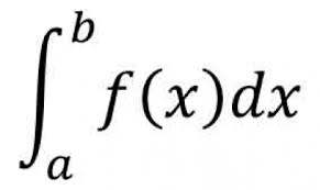
Image 1: Integral Notation
|
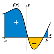
Image 2: Integral Visualization
|
Riemann Sums
Riemann sums are approximations of integrals. It is taken by adding the areas of calculable shapes at certain intervals. As the interval values get smaller, the Riemann Sum gets more precise. As the limit of the interval length approaches 0, you get an actual integral. The three simplest Riemann Sums are Left Riemann Sums, Midpoint Riemann Sums, and Right Riemann Sums. Here, the sums are taken exactly as they sound, the Left Riemann Sum by the value to the left of the interval, the Midpoint Riemann Sum by the midpoint of the interval, and the Right Riemann Sum by the right value of the interval (as illustrated by Images 3, 4, and 5, respectively). As you can see, no matter which method you use, there will always be a margin of error. In the Left Riemann Sum, when the graph is increasing, there will be an underestimation and an overestimation if the graph is decreasing. For the Right Riemann Sum, the exact opposite happens; there is an overestimation for increasing sections of the graph and an underestimation for decreasing sections of the graph. The Midpoint Riemann Sum tends to be a bit more accurate, but over-/under-estimates are difficult to tell.
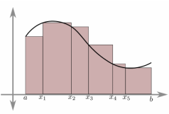
Image 3: Left Riemann Sum
|
Image 4: Midpoint Riemann Sum
|
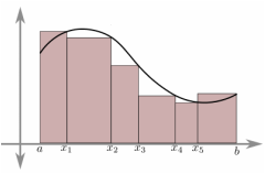
Image 5: Right Riemann Sum
|
Another two, more difficult, versions of Riemann sums are the Trapezoidal Rule and Simpson's Rule. These, while more accurate usually take longer to calculate. The Trapezoidal Rule is calculated by replacing the rectangles of a Riemann Sum with trapezoids. Simpson's Rule is calculated by replaces the top of the rectangle with a parabolic cap, and while it is the hardest of Riemann Sums, it is also the most accurate method of approximation.
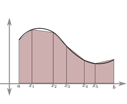
Image 6: Trapezoidal Rule
|
Image 7: Simpson's Rule
|
